
Here we review the equations that represent the physical laws governing atmospheric motion. Rigorous derivations of the equations may be found in many text books, such as Gill (1982) and Holton (2004).
The motion of an air parcel is governed by Newton's second law of motion, which states that the acceleration of the parcel equals the force per unit mass that acts upon it. For large-scale geophysical flows on a rotating planet, a rotating coordinate system is used because the fluid as a whole rotates with constant angular velocity and it is the fluid motion relative to the bulk rotation that is most relevant and useful for the prediction of atmospheric flow. In a uniformly rotating frame of reference pseudo forces (Coriolis and centrifugal forces) must be added to Newton's equation so as to account for the accelerating (non-inertial) frame of reference. In the rotating reference frame, Newton's second law can be expressed mathematically as follows:
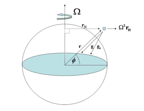
where u is the velocity of the air parcel, ρ is its density, p is the pressure, Ω is the angular rotation vector of the reference frame (e.g. the Earth), F is the frictional force per unit mass acting on the parcel, t is the time, and ge is the "effective" gravitational acceleration. The "effective" gravitational acceleration is the vector sum of the acceleration due to gravity and the pseudo force associated with the centripetal acceleration arising from the Earth's rotation

where rH denotes the component of the parcel's position vector r that is perpendicular to Ω (see Fig. 1.1) and φe is the effective gravitational potential. The centripetal term is usually written as minus the gradient of a centrifugal potential (Ω2rH2/2) and lumped with the ordinary gravitational potential (φ) to give an effective gravitational potential (φe). For terrestrial flows the centripetal acceleration is approximately 0.3% that of gravity. Hereafter the 'e' subscript will be dropped unless otherwise noted.
The material derivative D/Dt is calculated following the air parcel in the rotating coordinate system and has the form

In the case of a fluid at rest, u = 0 and the momentum equation reduces to

This equation expresses hydrostatic equilibrium and is a form of the hydrostatic equation. When expressed in a rectangular or cylindrical coordinate system with z pointing upwards, g = (0,0,-g) and Eq. (1.4) takes the more familiar form

Equations (1.4) and (1.5) are called the hydrostatic equation because they express a balance between the vertical pressure gradient and the gravitational force, both per unit volume, a state that we call hydrostatic balance.
The motion of the air described by (1.1) is subject to the constraint that at every point in the flow, mass must be conserved. In general, for a compressible fluid such as air, mass conservation is expressed by the equation

We call this the continuity equation.
In practice, density fluctuations in the air are rather small and can be neglected unless we want to study sound propagation or buoyancy effects. Usually, shallow layers of air on the order a kilometre deep or less can be considered to be homogeneous (ρ = constant) to a first approximation and therefore incompressible. In this case the continuity equation reduces to

This approximation is formally not accurate for deeper layers since air is compressible under its own weight. For example, the density at a height of 10 km is only about a quarter of that at mean sea level. Even so, for some purposes this pseudo-incompressible approximation to the continuity equation often suffices for qualitative insight even when buoyancy effects are considered. When the density fluctuations are small their impact in both the continuity and momentum equations can be neglected everywhere except where they multiply the gravitational acceleration. This is the so-called Boussinesq approximation. In situations where further accuracy is desired one may still neglect the time and horizontal variations of density in the continuity and momentum equations, but retain the vertical variation of the density field. In (1.6) one then sets ρ = ρo(z), where ρo(z) is the mean density at a particular height z, whereupon (1.6) becomes

This equation forms part of what is called the anelastic approximation in which the density is allowed to vary only with height.
The constraint imposed by (1.7) or (1.8) means that the formulation of fluid flow problems in enclosed regions is intrinsically different to that for problems in rigid body dynamics. In the latter, a typical problem is to specify the forces acting on a body and calculate its resulting acceleration. In many fluid flow problems, the force field cannot be imposed arbitrarily: it must produce accelerations that are compatible with ensuring mass continuity at all times. In general, this means that the pressure field cannot be arbitrarily prescribed: it must be determined as part of the solution. Thus methods for solving fluid flow problems are different also from those those required for solving rigid-body problems (see section 1.6).
For homogeneous fluids, Eqs. (1.1) and (1.7) suffice to determine the flow when suitable initial and boundary conditions are prescribed. However, when density varies with pressure and temperature we need additional equations: a thermodynamic equation and an equation of state. The latter is a relationship between the pressure, density and absolute temperature, T, of the parcel. For dry air the ideal gas equation ordinarily suffices to a high level of accuracy for most atmospheric flows

where Rd is the specific gas constant for dry air.
There are various forms of the thermodynamic equation, which is an expression of the first law of thermodynamics. This law states that the amount of heat added to an air parcel per unit mass, dq, equals the change in internal energy per unit mass, du, plus the amount of work done by the parcel, dw, in expanding against its environment. For a two parameter system (dry air is governed by two state variables) dw equals the pressure times the change in specific volume, dα. The specific volume is the volume per unit mass and is equal to the inverse of the density. For dry air, du = cvddT, where cvd is the specific gas constant for dry air at constant volume. Then the first law takes the form:

Using the equation of state and the fact that α = 1/ρ, Eq. (1.10) may be written as

where cpd = cvd + Rd is the specific gas constant for dry air at constant pressure. Equation (1.11) may be rewritten more succinctly as

where κ = Rd / cpd. When applied to a moving air parcel, Eq. (1.12) may be written in the form

For dry air, Eqs. (1.1), (1.6), (1.9), (1.13) form a complete set to solve for the flow, subject to suitable initial and boundary conditions.
Two alternative forms of (1.13) are frequently used. It is common to define the potential temperature, θ, as T(p**/p)κ, where p** is a reference pressure, normally taken to be 1000 mb (or 1 hPa). Then (1.13) becomes

where π = (p**/p)κ, is called the Exner function. If there is no heat input into an air parcel during its motion, the right-hand-side of (1.14) is zero, implying that θ remains constant for the parcel in question. A process in which there is no external heat source or sink is called an adiabatic process. The potential temperature may be interpreted as the temperature that an air parcel with temperature T at pressure p would have if it were brought adiabatically to a standard reference pressure, p**. Diabatic processes are ones in which the heating rate following the parcel, Dq/Dt, is non zero.
A second common form of (1.13) is

where s = cpd ln θ is known as the specific entropy of the air.
Equation (1.5) can be written in differential form as dp = - ρgdz, or dp = - dφ, whereupon (1.10) becomes dq = cpddT + dφ . In this situation, an alternative equation expressing the first law of thermodynamics is

where hd = cpdT + dφ is known as the dry static energy of the air.
Equations of the type (1.1), (1.6), (1.14) or (1.14) that involve time derivatives are called prediction equations, because they can be integrated in time (perhaps not analytically) to forecast subsequent values of the dependent variable in question. In contrast, equations such as (1.4), (1.5), (1.7), (1.8), and (1.9) are called diagnostic equations, because they give a relationship between the dependent variables at a particular time, but involve time only implicitly.
Equations (1.13)-(1.16) hold to a good first approximation even when the air contains moisture, in which case a dry adiabatic process is one in which the air remains unsaturated. However, tropical cyclones owe their existence to moist processes and the inclusion of these in any theory requires an extension of the foregoing equations to allow for the latent heat that is released when water vapour condenses or liquid water freezes and which is consumed when cloud water evaporates or ice melts. We require also equations characterizing the amount of water substance in the air and its partition between the possible states: water vapour, liquid water and ice.
Water content is frequently expressed by the mixing ratio, the mass of water per unit mass of dry air. We denote the mixing ratios of water vapour, liquid water, ice, and total water by r, rL, ri and rT, respectively. Sometimes specific humidity, q, is used rather than r. It is defined as the mass of water per unit mass of moist air and related to r by q = r/(1 + r). Since, in practice, r << 1, the difference between r and q is not only small, but barely measurable.
The equation of state for air containing water vapour as well as hydrometeors (liquid water drops, ice crystals) may be written as

where Tρ is a fictitious temperature, the density temperature, defined by

where ε = 0.622 is the ratio of the specific heat of dry air to that for water vapour and rT is the mixing ratio of water substance (i.e. water vapour, liquid water and ice). The use of Tρ in Eq. (1.17) is an artifice that enables us to retain the specific heat for dry air in the equation. The alternative would be to use a specific gas constant for the mixture of air and water substance that would depend on the mixing ratios of these quantities (i.e. it would not be a constant!). In the special case when there are no hydrometeors in the air, the density temperature reduces to the virtual temperature, Tv, which may be written approximately as T(1 + 0.61r).
The extension of the thermodynamic equation to include water substance and the equations for the various species of water substance will be delayed until Chapter 6. Suffice it to say here that the introduction of various states of water requires a modification of the equation to account for the latent heat released or consumed during phase changes of water substance. Additional equations governing the rates-of-change of the mixing ratios for water vapour, liquid water and ice as well as conversions between these states are required also.
Vorticity is defined as the curl of the velocity vector and we denote it by ω: i.e. ω = ∇ ∧ u. For a body of fluid rotating as a solid body, the vorticity vector is oriented along the axis of rotation in a direction such that the rotation is counter clockwise and it has a magnitude equal to twice the angular rotation rate. In general, vorticity is a measure of the local rotation rate of a parcel of fluid. Not surprisingly, vorticity is an important concept for characterizing rotating flows such as tropical cyclones and other geophysical vortices including tornados, waterspouts and dust devils.
We may derive an equation for ω simply by taking the curl of the momentum equation (1.1). The resulting equation, the Helmholtz vorticity equation, takes the general form

The quantity ω: + 2Ω is called the absolute vorticity and is the sum of the relative vorticity, ω, i.e. the curl of the velocity vector relative to a coordinate system rotating with angular velocity Ω, and the background vorticity, 2Ω, the vorticity associated with the rotating coordinate system. The term on the left-hand-side is simply the rate-of-change of vorticity following a fluid parcel. The terms (ω + 2Ω) ⋅ ∇ u can be interpreted as the rate-of-production of vorticity as a result of the stretching and bending of absolute vorticity by velocity gradients. The term (1/ρ2) ∇ρ ∧ ∇p represents the baroclinic generation of vorticity and the term ∇ ∧ F is the frictional generation term.
For a homogeneous fluid, or for so-called barotropic flows in which the pressure is a function of density alone, the second term on the right-hand-side of (1.19) is zero. In such cases the vorticity equation does not involve the pressure. This feature has advantages for interpretation because, as noted in section 1.6}, pressure cannot be prescribed arbitrarily, but must be determined as part of the solution. Thus, in these cases, interpretations in terms of vorticity circumvent the need to know about the pressure field and are often easier to conceptualize than those based directly on the momentum equation.
A class of flows in which we will have interest are homogeneous or barotropic, frictionless and two-dimensional in planes perpendicular to the axis of rotation. In such flows, the vorticity equation reduces to

where, in this case, ω and Ω are scalar quantities. Then, the absolute vorticity of air parcels (or in this case air columns), ω + 2Ω, is conserved as these air parcels move around.
Another quantity that will prove useful in understanding certain types of flow is the Ertel potential vorticity, P, defined as

For the general adiabatic motion of a rotating stratified fluid, P is conserved for fluid parcels, i.e.,

When diabatic and/or frictional effects are present, P is no longer materially conserved, but is governed by the equation

dot θ is the diabatic heating rate given by the right-hand-side of (1.14), K represents the curl of the frictional force F per unit mass (i.e. K = ∇ ∧ F) and

Equation (1.23) shows that diabatic heating in a localized region produces a dipole anomaly of potential vorticity with its axis oriented along the absolute vorticity vector (ω + 2Ω) and in the opposite direction to it (Fig. 1.2a). Cooling instead of heating reverses the direction of the dipole (Fig. 1.2b).
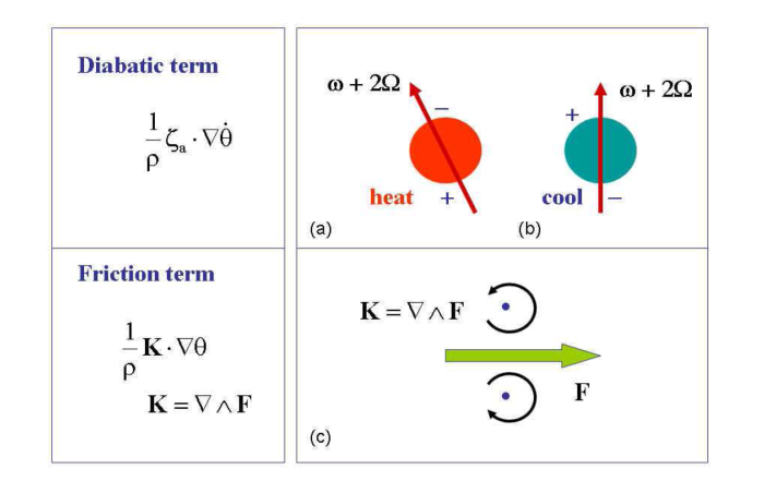
The action of a localized force F produces positive relative vorticity to its left and negative relative vorticity to its right (Fig. 1.2c), at a rate K equal to ∇ ∧ F. Recalling that P = (1/ρ )( {ω + 2Ω ) ⋅ ∇ θ and recalling that the frictional generation term in (1.23) has the form (1/ρ )∇ ∧ F ⋅ ∇ θ, we see how the latter contributes to a change in and hence a change in (1/ρ ){ω + 2Ω ) ⋅ ∇ θ. Note that again, a localized force produces a dipole anomaly of potential vorticity, being the projection of the dipole anomaly of (ω + 2Ω), i.e. ∇ ∧ F, on the potential temperature gradient, ∇ θ.
When integrated over a region of space V, Eq.(1.23) gives

where S is the surface of V and hat n is the unit normal to S, outward from V.
An important result that follows from (X.24) is that purely internal diabatic heating or friction cannot change the mass-weighted potential vorticity distribution within V, i.e., if dot θ and K are zero on S, then

Thus internal diabatic heating or friction can only redistribute the mass-weighted potential vorticity that is there.
The momentum equations (1.1), the thermodynamic equation (1.13) or one of its equivalent forms (Eqs. (1.14) or (1.15)), the equation of state (1.9), and the continuity equation (1.2) or one of the approximations to it (Eqs. (1.7) or (1.8)) form a complete set for solving problems of dry air flow. For moist air flows, the equation of state in the form (1.17) must be used and additional equations are necessary to characterize the various species of water substance. The set of equations is referred to as the primitive equations. The equations are rather general and admit a wide range of solutions. If the density is allowed to vary with space and time, the general solutions include motions associated with sound waves as well as range of wave types. The solutions are greatly constrained by the boundaries of the flow domain. For example, at an impervious boundary, there can be no component of flow normal to the boundary. If the fluid is considered to be inviscid, there can be no stress along the boundary and the flow adjacent to the boundary must be tangential to it. An inviscid fluid is an idealization in which the internal viscosity is zero. Such a fluid cannot support shearing stresses. If the fluid is viscous, there can be no flow at the boundary, but gradients normal to the boundary of flow parallel to the boundary may be large if the fluid viscosity is small. At a free surface, such as a water surface, the pressure is often taken to be constant at the surface if surface tension effects can be neglected.
As noted in section xx, the assumption that the fluid is incompressible or anelastic and enclosed by impervious boundaries means that the pressure distribution cannot be imposed arbitrarily, but must be determined as part of the solution. For this reason, arguments for explaining flow behaviour on the basis of prescribed forces, as in rigid body dynamics, are usually not possible. However in many flow situations, other methods of solution are possible and some can provide powerful insights into the flow behaviour. One such method, used widely in two-dimensional problems, is the vorticity-streamfunction approach. This approach exploits the fact that one can define a streamfunction that satisfies the continuity equation exactly and that there is only one component of vorticity, that normal to the plane of flow, which may be expressed in terms of the streamfunction. The simplest case is when the fluid is homogeneous, then one has just one pair of equations to solve: a prediction equation for the vorticity and a diagnostic equation for the streamfunction, neither of which involves the pressure explicitly. This method will be exploited later to gain an understanding of tropical cyclone motion.
For flows in which the density fluctuations are important, one needs a prediction equation for the thermodynamic equation as well. Moreover, in this case the vorticity equation involves also the pressure. Methods similar to the vorticity-streamfunction approach can nonetheless be devised for what are called balanced flows. These methods are based on a prediction equation for the potential vorticity or some asymptotic approximation to it and diagnostic relationships between streamfunction and/or dynamic pressure and the potential vorticity.
The foregoing equations are formulated independent of a particular coordinate system, but it is often convenient to use a rectangular coordinate system or cylindrical coordinate system with one direction, usually the z-direction, being in the local vertical direction at a particular latitude. Since tropical cyclones are relatively shallow circulations compared to their horizontal extent and because their horizontal extent is small compared with the radius of the Earth, we can safely approximate the Earth's surface as locally flat. Common rectangular coordinate systems for tropical cyclones have the x-axis pointing eastwards and the y-axis pointing northwards, or use cylindrical coordinates (r,λ,z) with r measuring radial distance from the coordinate axis and λ, the azimuthal angle, measured anticlockwise from east. It is usually only the vertical component of the Earth's rotation that is of consequence and it is customary to replace 2Ω by f, equal to 2|Ω|sin φ z, where φ is the latitude and z is a unit vector pointing locally upwards at the latitude of the origin of the coordinates. The quantity f is called the Coriolis parameter. When f is treated as a constant, we refer to such a coordinate system as an f-plane. There is a simple and useful generalization of this approximation for flows possessing somewhat larger horizontal length scales in which the variation of f with latitude cannot be neglected, but the explicit curvature of the earth's surface can still be safely ignored. In this circumstance the fluid equations using either Cartesian or cyclindical coordinates may be adopted with the simple modification of retaining a linear dependence of f with latitude. We refer to this coordinate system as a β-plane and write in Cartesian coordinates f = fo + βy, where fo is the value of f at the origin of the coordinates, and β = df/dy = 2Ω cosφo/a, where a is the Earth's mean radius.
In some problems it is convenient to use a vertical coordinate other than height. Common choices are:
the pressure;
the logarithm of the pressure;
the pseudo-height Z, which is a function of pressure that reduces to the actual height in an atmosphere with a uniform potential temperature;
the potential temperature; or
σ, which is defined either as the ratio of pressure to its surface value, or the pressure minus some upper-level pressure divided by the surface value minus this upper-level pressure.
Since the potential temperature and dry entropy are uniquely related, coordinates with θ in the vertical are called isentropic coordinates. In this case, for example, the potential vorticity takes a particularly simple form:

Now the scalar product no longer appears. Moreover, when expressed in these coordinates, the vertical advection in the derivative D/Dt is proportional to the heating rate (see Eq. (1.14)). For adiabatic motion, when Dθ/Dt = 0, (1.22) says that P is conserved on isentropic surfaces. This turns out to be a very useful result and will be exploited in these lectures.
It is common experience that air that is warmer than its surroundings rises and air that is colder sinks. This tendency may be quantified in terms of the buoyancy force. The buoyancy force that acts on an air parcel of volume V with density ρ in an environment with density ρa is defined as the difference between the weight of air displaced by the parcel, ρagV, (the upward thrust according to Archimedes' principle), and the weight of the parcel itself ρgV. This quantity is normally expressed per unit mass of the air parcel under consideration, i.e.

The calculation of the upward thrust assumes that the pressure within the air parcel is the same as that of its environment at the same level and that, ρa is the density of the environment at the same height as the parcel. Using the equation of state (1.9), the buoyancy force may be expressed alternatively in terms of temperature , b=g(T - Ta)/Ta, where T is the parcel temperature and Ta is the temperature of its environment. If the air contains moisture the virtual temperatures need to be used instead, while if the air contains condensate, the density temperature(s) must be used.. It follows that if an air parcel is warmer than its environment, it experiences a positive (i.e. upward) buoyancy force and tends to rise; if it is cooler, the buoyancy force is negative and the parcel tends to sink.
The tendency of warm air to rise is not immediately apparent from the vertical component of forces on the right-hand-side of the momentum equation (1.1). However, we can modify this equation so that a buoyancy term appears. We simply replace the pressure in this equation by the sum of a reference pressure pref, a function of height z only, and a perturbation pressure, p' = p - pref. The former is taken to be in hydrostatic balance with a prescribed reference density ρref, i.e. it satisfies Eq. (1.4). In idealized flows, the reference density is normally taken as the density profile in the environment, but in real situations, the environmental density is not uniquely defined. In these cases, ρref(z) could be taken as the horizontally-averaged density over some large domain surrounding the air parcel. Then Eq. (1.1) becomes

where b = bz.
A comparison of (1.1) and (1.26) shows that the sum of the vertical pressure gradient and gravitational force per unit mass acting on an air parcel is equal to the sum of the vertical gradient of perturbation pressure and the buoyancy force, where the latter is calculated from Eq. (1.25) by comparing densities at constant height. The expression for b in (1.26) has the same form as that in (1.25), but with ρref in place of ρa. However, the derivation circumvents the need to assume that the local (parcel) pressure equals the environmental pressure when calculating b. The pressure deviation is accounted for by the presence of the perturbation pressure gradient, the first term on the right-hand-side of (1.26).
The foregoing decomposition indicates that, in general, the buoyancy force is not uniquely defined because it depends on the (arbitrary) choice of a reference density. However, the sum of the buoyancy force and the vertical component of perturbation pressure gradient per unit mass s< unique. If the motion is hydrostatic, i.e. if the vertical acceleration is small compared with the gravitational acceleration, the perturbation pressure gradient and the buoyancy force are equal and opposite, but they remain non-unique.
We show later that the definition of buoyancy force requires careful consideration and some modification in a rapidly-rotating vortex.
Most atmospheric flows are turbulent, especially in regions of large wind shear, or in regions of vigorous buoyant convection. In such regions we attempt to predict the mean motion, but in order to do this we may need to take account of the diffusive properties of turbulent fluctuations. Sometimes this is done crudely by likening turbulent diffusion to molecular diffusion, but with a much larger coefficient of diffusion. Specifically we take F in Eq. (1.1) to be the vector K∇2u, where K is a so-called "eddy diffusivity"? associated with the turbulent fluctuations and u is the velocity vector. This analogy is crude because unlike molecular diffusion, where the diffusivity is a property of the fluid, K depends on the flow itself and treating it as a constant may be a poor assumption for quantitative calculations. Nevertheless, the assumption can be useful for elucidating the qualitative effects of turbulent momentum transfer, at least when that this transfer is downgradient.
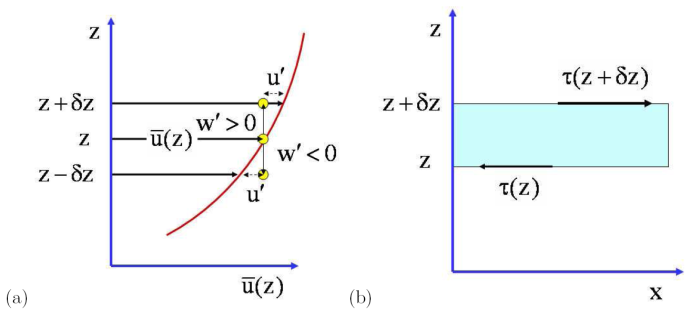
We illustrate the ideas for the case of a mean flow bar u(z) that is one dimensional in the x-direction (Fig. 1.8a). We assume that the total velocity at any height z is (bar u(z) + u', v', w'), where the prime quantities represent turbulent fluctuations that are functions of space and time, but have zero mean. We assume also that dbar u/dz > 0. In analogy to molecular diffusion we consider an air parcel at height z moving with the mean flow speed (i.e. u' = 0). Suppose that on account of the component of turbulent fluctuation w', it moves to the neighbouring level z + δz, conserving its linear momentum ρ bar u. If w' > 0, δz > 0 and at its new position the parcel will have a momentum deficit ρ u' = ρ(bar u(z) - bar u(z + δz), whereas if w' < 0, δz < 0 and it will have a momentum surplus. In both cases the quantity ρu'w' is negative and corresponds to a transport of x-momentum in the negative z-direction, i.e. in the opposite direction to the vertical gradient of bar u. Thus on average the mean lateral transport of momentum, ρ overline{u'w'}, is negative and hence downgradient, meaning down the gradient of bar u. We define K such that

The quantity τ = - ρ overline{u'w'} represents a mean turbulent transport, or flux, of x-momentum in the z-direction and is equivalent to a turbulent shear stress. A stress has units of force per unit area.
The force in the x-direction acting on a layer of fluid of thickness δz is proportional to the vertical gradient of the stress as indicated in Fig. 1.8b, i.e.

This expression is a special case in Cartesian coordinates of K∇2u = K(∇2u,∇2v,∇2w) when K is treated as a constant.
Similar expressions are obtained for other conserved scalar quantities, c. Suppose that bar c has a mean gradient d bar c/dz, then turbulent fluctuations give rise to a mean flux of c in the z-direction, Fc = -ρ overline{c'w'}. If d bar c/dz > 0, then the flux is normally ???? Unlike molecular diffusion, it is possible for a turbulent flux to be countergradient, in which case the eddy diffusivity would be negative. in the negative z-direction and we can write

where Kc is an eddy diffusivity for the quantity c. The rate of accumulation of c in a unit volume is simply minus the divergence of this flux in the volume.
Note that waves are associated also with fluctuations about a mean and the effects of waves on mean flows can be analysed in a similar way to those of turbulent fluctuations. For example there may be a stress associated with wave motions. Examples of this type will be discussed later.
Show that for a two-dimensional flow u = (u,v,0) in a rectangular coordinate system (x,y,z) with the rotation vector Ω = (0,0,Ω), Eq. (1.20) reduces to the scalar equation:

where ζ = ∂ v/ ∂ x - ∂ u/ ∂ y.
Consider the case of an axisymmetric vortex with tangential velocity distribution v(r), and assume a linear frictional force F = - μ v(r), μ (> 0) acts at the ground z = 0. Then K = - μ ζ k, where ζ is the vertical component of relative vorticity. Then PV is destroyed locally at the boundary at the rate (1/ρ )(K ⋅ ∇ θ ) = - (1/ρ )μ ζ (∂ θ /∂ z)_{z = 0}. The frictional force-curl term may be expected to be important in the boundary layer.
Using the gas law, p = ρ RdT, and the usual definition of virtual potential temperature, show that the buoyancy force per unit mass can be written as

where θ is the virtual potential temperature of the air parcel in K and θref is the corresponding reference value.
Note that the second term on the right-hand-side of (1.31) is sometimes referred to as the "dynamic buoyancy", but in some sense this is a misnomer since buoyancy depends fundamentally on the density perturbation and this term simply corrects the calculation of the density perturbation based on the virtual potential temperature perturbation.
Show that if the perturbation pressure gradient term in (1.26} is written in terms of the Exner function and/or its perturbation, the second term in (1.31) does not appear in the expression for buoyancy.
The x-momentum equation for the two-dimensional flow of a homogeneous, inviscid fluid in the x-z plane may be written

in standard notation. Assuming that the flow can be decomposed into a mean part and a fluctuating part, show that the mean flow satisfies the equation

where an overbar represents a mean quantity and a prime represents a fluctuation about the mean.
A. E. Gill, Atmosphere-Ocean Dynamics. Academic Press. 1982. 662pp.
J. R. Holton, An Introduction to Dynamic Meteorology. Academic Press. Fourth Edition. 2004. 529pp.
J. C. McWilliams. Fundamentals of geophysical fluid dynamics. Cambridge University Press, 2006, 272pp.
J. M. Wallace and P. V. Hobbs. Atmospheric Science: An introductory survey. Academic Press. Second Edition. 2006. 483pp.
C. F. Bohren and B. A. Albrecht. Atmospheric Thermodynamics. Oxford University Press. 1998. 402pp.
K. A. Emanuel. Atmospheric Convection. Oxford University Press. 1994. 580pp.
Hoskins, B. J., M. E. McIntyre, and A. W. Robertson, 1985: On the use and significance of potential vorticity maps. Quart. J. Roy. Meteor. Soc., 111, 877-946.
Latest version: Munich 21 July 2013